Tillandsia brachycaulos
BIOL4558
Agosto 2021
APPENDIX S1
- R code for figures
- This appendix provides R code for producing the figures included in the main manuscript.
- Install the library using install.packages() or by downloading from http://cran.R-project.org
Load the library ( some minor changes)
library(popdemo)
library(popbio)
Lectura
Deben leer el siguiente manuscrito para lunes, habrá prueba corta sobre este manuscrito.
Mondragón, Durán, Ramírez, Valverde. Habrá un quiz de comprobación de lectura al principio de la clase.
 Tis=matrix(c(
0,0,0,0.007,0.017,0.036,0,.001,0.011,0.024,0.035,
0.28,0.167,0,0,0,0,0,0,0,0,0,
0,.33,.189,0,0,0,0,0,0,0,0,
0,.103,.378,.134,0,0,0,0,0,0,0,
0,0,.081,.179,.066,0,0,0,0,0,0,
0,0,0.014,0,0.082,0,0,0,0,0,0,
0,.039,0.108,.448,.754,.940,0,.300,0.570,.985,1.243,
0,0,0,0,0,0,.033,.57,0,0,0,
0,0,0,0,0,0,.148,.183,.035,0,0,
0,0,0,0,0,0,.18,.207,.193,.037,0,
0,0,0,0,0,0,.115,.126,.175,.066,0
), byrow=TRUE, ncol=11)

Tis
## [,1] [,2] [,3] [,4] [,5] [,6] [,7] [,8] [,9] [,10] [,11]
## [1,] 0.00 0.000 0.000 0.007 0.017 0.036 0.000 0.001 0.011 0.024 0.035
## [2,] 0.28 0.167 0.000 0.000 0.000 0.000 0.000 0.000 0.000 0.000 0.000
## [3,] 0.00 0.330 0.189 0.000 0.000 0.000 0.000 0.000 0.000 0.000 0.000
## [4,] 0.00 0.103 0.378 0.134 0.000 0.000 0.000 0.000 0.000 0.000 0.000
## [5,] 0.00 0.000 0.081 0.179 0.066 0.000 0.000 0.000 0.000 0.000 0.000
## [6,] 0.00 0.000 0.014 0.000 0.082 0.000 0.000 0.000 0.000 0.000 0.000
## [7,] 0.00 0.039 0.108 0.448 0.754 0.940 0.000 0.300 0.570 0.985 1.243
## [8,] 0.00 0.000 0.000 0.000 0.000 0.000 0.033 0.570 0.000 0.000 0.000
## [9,] 0.00 0.000 0.000 0.000 0.000 0.000 0.148 0.183 0.035 0.000 0.000
## [10,] 0.00 0.000 0.000 0.000 0.000 0.000 0.180 0.207 0.193 0.037 0.000
## [11,] 0.00 0.000 0.000 0.000 0.000 0.000 0.115 0.126 0.175 0.066 0.000Draw the life history of the matrix
Use the package Rage
library(Rage)plot_life_cycle(Tis)isErgodic(Tis, digits=10, return.eigvec=FALSE)## [1] TRUEisIrreducible(Tis)## [1] TRUEeigs <- eigen(Tis)
eigs## eigen() decomposition
## $values
## [1] 0.80280104+0.00000000i -0.50597134+0.00000000i 0.49541679+0.00000000i
## [4] 0.20710796+0.09680538i 0.20710796-0.09680538i 0.16083386+0.00000000i
## [7] -0.12932219+0.00000000i 0.01369206+0.09063629i 0.01369206-0.09063629i
## [10] -0.05158780+0.00000000i -0.01577040+0.00000000i
##
## $vectors
## [,1] [,2] [,3] [,4]
## [1,] 0.0213778093+0i 2.199609e-02+0i -0.026611645+0i 0.01284490+0.01249956i
## [2,] 0.0094145593+0i -9.151807e-03+0i -0.022688427+0i 0.04399465-0.01892493i
## [3,] 0.0050615824+0i 4.345642e-03+0i -0.024434631+0i -0.03522731-0.15656289i
## [4,] 0.0043106658+0i -1.093825e-03+0i -0.032021751+0i -0.44576698-0.24590206i
## [5,] 0.0016036858+0i -2.730947e-04+0i -0.017957142+0i -0.58569126+0.00000000i
## [6,] 0.0002520729+0i -7.598299e-05+0i -0.003662715+0i -0.19632715+0.08118299i
## [7,] 0.8980480775+0i 9.399319e-01+0i -0.867840964+0i 0.14723168+0.19900789i
## [8,] 0.1273000602+0i -2.882768e-02+0i 0.383983903+0i -0.00799236-0.02022906i
## [9,] 0.2034472709+0i -2.473966e-01+0i -0.126345107+0i 0.15365587+0.06319600i
## [10,] 0.2967677993+0i -2.126685e-01+0i -0.220566335+0i 0.35278354+0.05690204i
## [11,] 0.2173705248+0i -9.314631e-02+0i -0.177804855+0i 0.32703217+0.01686758i
## [,5] [,6] [,7]
## [1,] 0.01284490-0.01249956i -0.0000453397+0i 0.006658047+0i
## [2,] 0.04399465+0.01892493i 0.0020588443+0i -0.006291305+0i
## [3,] -0.03522731+0.15656289i -0.0241218240+0i 0.006522104+0i
## [4,] -0.44576698+0.24590206i -0.3318936463+0i -0.006901625+0i
## [5,] -0.58569126+0.00000000i -0.6470561119+0i 0.003620175+0i
## [6,] -0.19632715-0.08118299i -0.3319966694+0i -0.003001525+0i
## [7,] 0.14723168-0.19900789i 0.1339719239+0i -0.739477872+0i
## [8,] -0.00799236+0.02022906i -0.0108050816+0i 0.034894888+0i
## [9,] 0.15365587-0.06319600i 0.1418577991+0i 0.627163982+0i
## [10,] 0.35278354-0.05690204i 0.3977655917+0i 0.029100907+0i
## [11,] 0.32703217-0.01686758i 0.4049083558+0i -0.239952298+0i
## [,8] [,9] [,10]
## [1,] 0.071119011+0.013322706i 0.071119011-0.013322706i 0.11421734+0i
## [2,] -0.085589963-0.074933585i -0.085589963+0.074933585i -0.14630668+0i
## [3,] 0.069586877+0.177032359i 0.069586877-0.177032359i 0.20068018+0i
## [4,] 0.143758186-0.383768211i 0.143758186+0.383768211i -0.32754049+0i
## [5,] -0.599703404+0.000000000i -0.599703404+0.000000000i 0.36036606+0i
## [6,] -0.051811255+0.523985070i -0.051811255-0.523985070i -0.62727112+0i
## [7,] -0.061801463+0.042517465i -0.061801463-0.042517465i 0.19520792+0i
## [8,] 0.003971536-0.001875061i 0.003971536+0.001875061i -0.01036356+0i
## [9,] 0.082898608+0.073407980i 0.082898608-0.073407980i -0.31175569+0i
## [10,] 0.206639886-0.115997988i 0.206639886+0.115997988i 0.30677677+0i
## [11,] 0.141282490-0.216296225i 0.141282490+0.216296225i 0.25523237+0i
## [,11]
## [1,] 0.002799353+0i
## [2,] -0.004288544+0i
## [3,] 0.006911250+0i
## [4,] -0.014493735+0i
## [5,] 0.024881465+0i
## [6,] -0.135509394+0i
## [7,] -0.112331807+0i
## [8,] 0.006328332+0i
## [9,] 0.304646450+0i
## [10,] -0.755859400+0i
## [11,] 0.551309967+0i lambdamax <- Re(eigs$values[1])
lambdamax## [1] 0.802801lambda(Tis)## [1] 0.802801truelambda(Tis)## [,1] [,2]
## [1,] 0.802801 0.8028011
## [2,] 0.802801 0.8028011
## [3,] 0.802801 0.8028011
## [4,] 0.802801 0.8028011
## [5,] 0.802801 0.8028011
## [6,] 0.802801 0.8028011
## [7,] 0.802801 0.8028011
## [8,] 0.802801 0.8028011
## [9,] 0.802801 0.8028011
## [10,] 0.802801 0.8028011
## [11,] 0.802801 0.8028011Stable stage Distribution
The relative proportion of individuals represented in each age/stage of an exponentially increasing (or decreasing) population. Once the populaiton reaches a stable age/stage distribution, these proportion remainconstant through time. A stage age/stage distribution implies that a population is growing with fixed survivorship lx and fecundity bx schedules.
What are the assumptions in regards to this concept?
Elaborate::::
w <- stable.stage(Tis)
w
## [1] 0.0119766716 0.0052743985 0.0028356933 0.0024150009 0.0008984465
## [6] 0.0001412209 0.5031211018 0.0713183939 0.1139789925 0.1662607447
## [11] 0.1217793353Reproductive value, vx
Reproductive value is the expected number of offspring that remain to be born to individuals of age/stage x. By definition the value of newborns v0 is 1.0.
v <- reproductive.value(Tis)
v
## [1] 1.000000 2.867147 3.830711 3.916761 4.624162 4.709649 3.983948
## [8] 18.134366 5.818338 5.691014 6.212058Elasticities and Sensitivity
Both of these tools let you understand the importance of the effect of growth/persistence of the population, and determine which of the parameters are most relevant to future growth.
Using the elasticity vs. the sensitivity.
Elasticity assesses effect of a proportional change in the values such as lambda: In other words if you were able modify the parameter (increase of decrease survivorship or reproduction) what would be the proportional effect on the growth of the population. In this case the values of reproduction and survivorhsip and growth are comparible (same scale)
sensitivities assess the effect of an additive change. Reproduction and survivorship and growth are on different scales.
sens(Tis)## [,1] [,2] [,3] [,4] [,5]
## [1,] 0.000000000 0.000000000 0.000000000 0.0004225115 0.0001571858
## [2,] 0.006007686 0.002645721 0.000000000 0.0000000000 0.0000000000
## [3,] 0.000000000 0.003534870 0.001900465 0.0000000000 0.0000000000
## [4,] 0.000000000 0.003614275 0.001943155 0.0016548763 0.0000000000
## [5,] 0.000000000 0.000000000 0.002294106 0.0019537617 0.0007268529
## [6,] 0.000000000 0.000000000 0.002336517 0.0000000000 0.0007402901
## [7,] 0.000000000 0.003676273 0.001976488 0.0016832636 0.0006262202
## [8,] 0.000000000 0.000000000 0.000000000 0.0000000000 0.0000000000
## [9,] 0.000000000 0.000000000 0.000000000 0.0000000000 0.0000000000
## [10,] 0.000000000 0.000000000 0.000000000 0.0000000000 0.0000000000
## [11,] 0.000000000 0.000000000 0.000000000 0.0000000000 0.0000000000
## [,6] [,7] [,8] [,9] [,10] [,11]
## [1,] 2.470702e-05 0.0000000 0.01247736 0.01994096 0.0290878 0.02130565
## [2,] 0.000000e+00 0.0000000 0.00000000 0.00000000 0.0000000 0.00000000
## [3,] 0.000000e+00 0.0000000 0.00000000 0.00000000 0.0000000 0.00000000
## [4,] 0.000000e+00 0.0000000 0.00000000 0.00000000 0.0000000 0.00000000
## [5,] 0.000000e+00 0.0000000 0.00000000 0.00000000 0.0000000 0.00000000
## [6,] 0.000000e+00 0.0000000 0.00000000 0.00000000 0.0000000 0.00000000
## [7,] 9.843146e-05 0.0000000 0.04970915 0.07944373 0.1158843 0.08488060
## [8,] 0.000000e+00 1.5962324 0.22626904 0.00000000 0.0000000 0.00000000
## [9,] 0.000000e+00 0.5121447 0.07259751 0.11602323 0.0000000 0.00000000
## [10,] 0.000000e+00 0.5009373 0.07100884 0.11348427 0.1655391 0.00000000
## [11,] 0.000000e+00 0.5468010 0.07751010 0.12387439 0.1806951 0.00000000Elasticities
elas(Tis)## [,1] [,2] [,3] [,4] [,5]
## [1,] 0.000000000 0.0000000000 0.000000e+00 3.684076e-06 3.328545e-06
## [2,] 0.002095354 0.0005503672 0.000000e+00 0.000000e+00 0.000000e+00
## [3,] 0.000000000 0.0014530464 4.474182e-04 0.000000e+00 0.000000e+00
## [4,] 0.000000000 0.0004637143 9.149374e-04 2.762246e-04 0.000000e+00
## [5,] 0.000000000 0.0000000000 2.314678e-04 4.356289e-04 5.975614e-05
## [6,] 0.000000000 0.0000000000 4.074638e-05 0.000000e+00 7.561498e-05
## [7,] 0.000000000 0.0001785930 2.658948e-04 9.393387e-04 5.881532e-04
## [8,] 0.000000000 0.0000000000 0.000000e+00 0.000000e+00 0.000000e+00
## [9,] 0.000000000 0.0000000000 0.000000e+00 0.000000e+00 0.000000e+00
## [10,] 0.000000000 0.0000000000 0.000000e+00 0.000000e+00 0.000000e+00
## [11,] 0.000000000 0.0000000000 0.000000e+00 0.000000e+00 0.000000e+00
## [,6] [,7] [,8] [,9] [,10] [,11]
## [1,] 1.107937e-06 0.00000000 1.554228e-05 0.0002732315 0.0008695894 0.00092887
## [2,] 0.000000e+00 0.00000000 0.000000e+00 0.0000000000 0.0000000000 0.00000000
## [3,] 0.000000e+00 0.00000000 0.000000e+00 0.0000000000 0.0000000000 0.00000000
## [4,] 0.000000e+00 0.00000000 0.000000e+00 0.0000000000 0.0000000000 0.00000000
## [5,] 0.000000e+00 0.00000000 0.000000e+00 0.0000000000 0.0000000000 0.00000000
## [6,] 0.000000e+00 0.00000000 0.000000e+00 0.0000000000 0.0000000000 0.00000000
## [7,] 1.152534e-04 0.00000000 1.857589e-02 0.0564061640 0.1421846942 0.13142307
## [8,] 0.000000e+00 0.06561485 1.606542e-01 0.0000000000 0.0000000000 0.00000000
## [9,] 0.000000e+00 0.09441619 1.654874e-02 0.0050583058 0.0000000000 0.00000000
## [10,] 0.000000e+00 0.11231763 1.830943e-02 0.0272825547 0.0076294698 0.00000000
## [11,] 0.000000e+00 0.07832839 1.216525e-02 0.0270029781 0.0148553353 0.00000000TRANSIENT DYNAMICS
Fig. 2a: Population-specific transient dynamics # This figure is designed to be 3.5” by 3.5” (Check size of plot window using ‘par(din)’).
Set margins:
par(mar=c(10,4,1,1))#Create 2 population vectors. One is adult- #biased, and it amplifies. One is juvenile- # biased and it attenuates.
n0.amp <- c(1000,1,1,1,1,1,1,1,1,1,1)

n0.att <- c(1,1,1,1,1,1,1,1,1,1,1000)
Project these vectors using the project function. We are standardising the matrix using ‘standard.A=T’ to remove effects of asymptotic dynamics. This means that the projection has a long-term growth rate of unity, i.e. it does not grow or decline in the long-term. We also standardise the population vector to sum to 1 using ‘standard.vec=T’. These standardisations make it easier (and fairer) to compare between models with different population sizes, and different long-term growth rates.
pr2.1 <- project(Tis, vector=n0.amp, time=156,
                 standard.A=T, standard.vec=T)
pr2.2 <- project(Tis, vector=n0.att, time=156,
                 standard.A=T, standard.vec=T)
Plot the amplification projection and label it
plot(pr2.1, ylim=c(0.4,1), log="y", cex.axis=0.8)
text(52, pr2.1[51], "amplification",
     adj=c(1,-0.5), cex=0.8)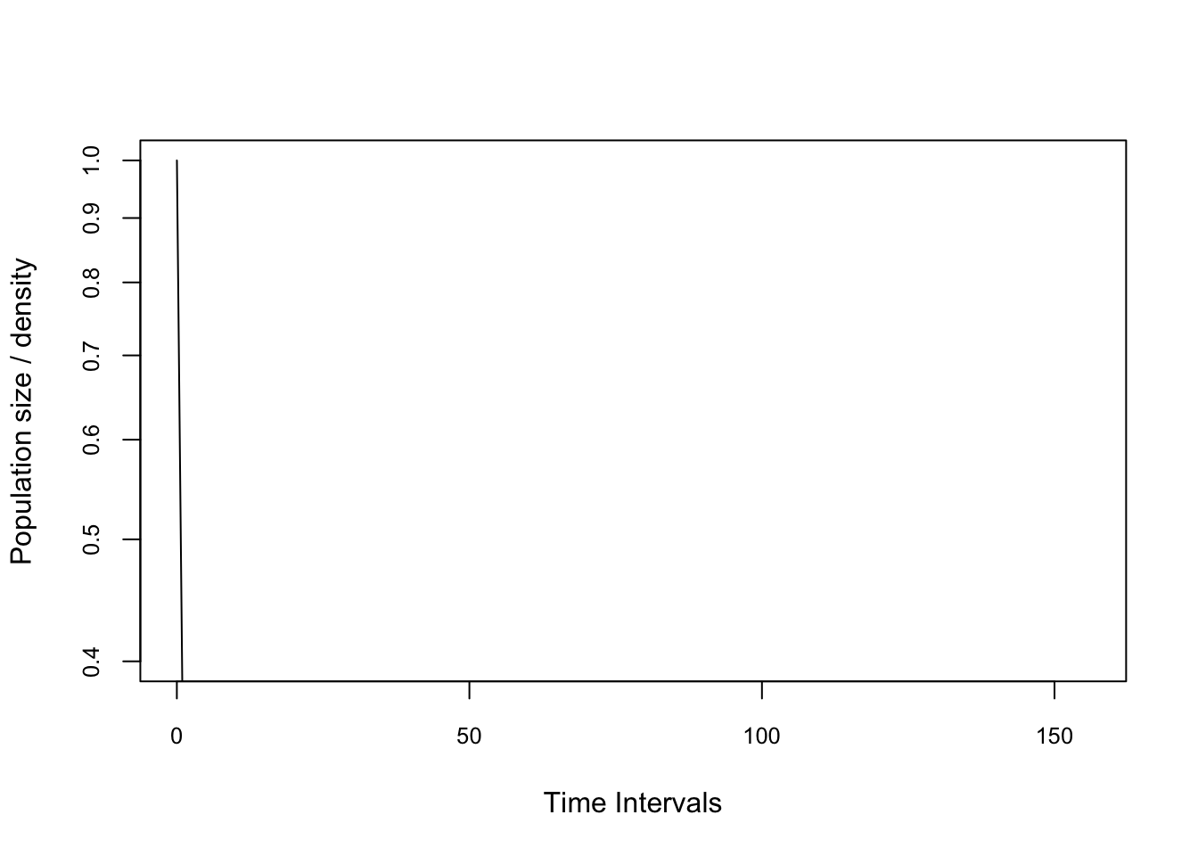
#maxamp(Tis, vector=n0.amp)
reac(Tis,vector=n0.amp)
## [1] 0.3568064inertia(Tis,vector=n0.amp)## [1] 0.1835773Calculate the transient dynamics of the amplification projection
reac <- reac(Tis, vector=n0.amp)
#maxamp <- maxamp(Tis, vector=n0.amp, return.t=T)
upinertia <- inertia(Tis, vector=n0.amp)
Add points on the projection for amplification and label them
#points(c(1,maxamp$t,31), c(reac,upinertia),
#       pch=3, col="red")
#text(1, reac, expression(bar(P)[1]),
#     adj=c(-0.3,0.5), col="red", cex=0.8)
#text(maxamp$t, maxamp$maxamp, expression(bar(P)[max]),
 #    adj=c(0.1,-0.5), col="red", cex=0.8)
#text(31, upinertia, expression(bar(P)[infinity]),
#     adj=c(0.1,-0.5), col="red", cex=0.8)
Add in the second projection using the ‘lines’ command and label it lines(0:50, pr2.2) text(52, pr2.2[51], “attenuation”, adj=c(1,1), cex=0.8)
Calculate the transient dynamics of the attenuation projection firstep <- firststepatt(Lrub1, vector=n0.att) maxatt <- maxatt(Lrub1, vector=n0.att, return.t=T) lowinertia <- inertia(Lrub1, vector=n0.att)
firststepatt(Lrub1, vector=n0.att) maxatt(Lrub1, vector=n0.att, return.t=T) inertia(Lrub1, vector=n0.att)
Add points on the attenuation projection and label them points(c(1,maxatt\(t,31), c(firstep,maxatt\)maxatt,lowinertia), pch=3, col=“red”) text(1, firstep, expression(underline(P)[1]), adj=c(0,-0.6), col=“red”, cex=0.8) text(maxatt\(t, maxatt\)maxatt, expression(underline(P)[min]), adj=c(0.1,1.5), col=“red”, cex=0.8) text(31, lowinertia, expression(underline(P)[infinity]), adj=c(0.1,1.5), col=“red”, cex=0.8)
Add in a dotted line at y=1 lines(c(0,50),c(1,1),lty=2)
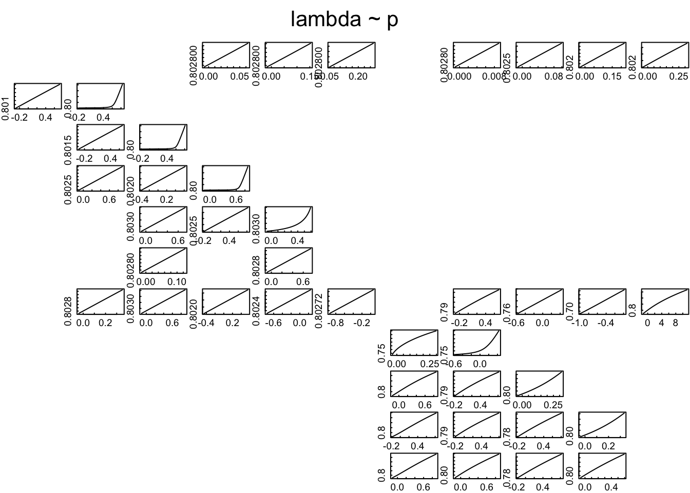
FIGURE 4: TRANSFER FUNCTION MATRIX
This figure is designed to be 7” by 7” (Check size of plot window using ‘par(din)’).
This is a nice, easy plot because the function does it all for you. The functions ‘tfmat’ and ‘inertia.tfmat’ calculate a transfer function for every PPM element. They are saved as arrays of values. The functions are customisable: see ‘?tfmat’ and ‘?inertia.tfmat’.
Create the array for inertia, using a specific population vector: n0 <- c(48, 16, 12, 10) tfmat <- inertia.tfamatrix(Lrub1, vector=n0)
…and plot it! plot(tfmat)
n0 <- c(48, 16, 12, 10)
tfmat <- tfamatrix(Tis)
## Warning in tfamatrix(Tis): 'tfamatrix' has been renamed and is deprecated.
## The old name will continue to work for now, but may be removed in later versions.
## Use the new name 'tfam_lambda' instead. See help("popdemo-deprecated") for more info.#...and plot it!
plot(tfmat)